


Next: What Statistical Power Means
Up: Formal Questions of a
Previous: Probability Distributions
Index
Click for printer friendely version of this HowTo
Imagine that the teacher mentioned in the previous section was indeed
attempting to determine if the study session he held two days before
the exam helped or not. One potential pitfall in simply visually
comparing to graphs would be that an improvement in scores could be
due to several factors, not just to the study session. For example,
this year's class, as a whole, could have been luckier in the multiple choice
section than the previous year's. Is there any way to characterize
how lucky a class would need to be in order to perform much better?
If there was (and there is), then perhaps the teacher could interpret
the fact that the class would have to be amazingly lucky to perform as
well as is did as not just luck, but due to his study session.
In a sense, the fundamental idea in statistics is to try to determine
if change is a result of chance or due to a specific reason. In order
to do this, we must consider variability (see Figures 3.2.2,
3.2.3 and 3.2.4).
Figure:
Two normal pdfs. One with mean = 0, or  , and the other with
 . Both
have the same variance,
. Both
have the same variance,
 . Notice that with a small amount of
variance, the two graphs hardly overlap and it is easy to distinguish
how one is fundamentally different from the other.
. Notice that with a small amount of
variance, the two graphs hardly overlap and it is easy to distinguish
how one is fundamentally different from the other.
![\includegraphics[width=3in]{normal}](img482.png) |
Figure:
Two normal pdfs. One with and the other with . Both
have the same variance,
 . Notice how with the increased
variance, the two curves overlap each other more than in Figure 3.2.2.
. Notice how with the increased
variance, the two curves overlap each other more than in Figure 3.2.2.
![\includegraphics[width=3in]{normal2}](img483.png) |
Figure:
Two normal pdfs. One with and the other with . Both
have the same variance,
 . Compare the variance and the
overlap with Figures 3.2.2 and 3.2.3. The more
overlap there is, the harder it is to determine if they are
fundamentally different.
. Compare the variance and the
overlap with Figures 3.2.2 and 3.2.3. The more
overlap there is, the harder it is to determine if they are
fundamentally different.
![\includegraphics[width=3in]{normal3}](img484.png) |
The variance of a model, notated with  , quantifies how
spread out the data is. In Figures 3.2.2, 3.2.3 and
3.2.4 we can see how larger values for result in
shorter peaks and a broader distribution of the data. If we can
determine the variance for a model (usually it is estimated from the
data), then we can use this information to help calculate the
significance of the
difference between two samples. Typically, this is done by
calculating difference between the two sample means and dividing by
the square root of the variation. That is,
, quantifies how
spread out the data is. In Figures 3.2.2, 3.2.3 and
3.2.4 we can see how larger values for result in
shorter peaks and a broader distribution of the data. If we can
determine the variance for a model (usually it is estimated from the
data), then we can use this information to help calculate the
significance of the
difference between two samples. Typically, this is done by
calculating difference between the two sample means and dividing by
the square root of the variation. That is,
 |
(3.2.1) |
where
 is the mean of the
  data set,
 is the mean of the
  data set and
  is an estimate of the
variation in the distributions that the data came from, . We will talk
more about how to calculate shortly.
is an estimate of the
variation in the distributions that the data came from, . We will talk
more about how to calculate shortly.
If you think about it briefly, you will see that the smaller the variation, the more
significant the difference will be. Another way to think about it is
that, for data sets with large amounts of variation, the difference
between the two means must be greater in order to avoid being in the
area of overlap between the two distributions (Figure 3.2.4).
The Study Sessionno_title
For example, if the average exam score for the
year without the study session was 75%, thus,
 and the
and for the year with the study session
and the
and for the year with the study session
 , then the
difference the two years is,
, then the
difference the two years is,
 . If the
estimated variation in the distributions that the data came from is
. If the
estimated variation in the distributions that the data came from is  , then we will have
distributions like that seen in Figure 3.2.2 and the difference
between the two means would be quite clear. However, if
, then the difference would be scaled by Equation 3.2.1 to
be only 2, and not as significant.
, then we will have
distributions like that seen in Figure 3.2.2 and the difference
between the two means would be quite clear. However, if
, then the difference would be scaled by Equation 3.2.1 to
be only 2, and not as significant.

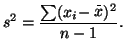
Calculating , an estimate of is quite simple. We
simply average the squared differences between
each observation and the mean. That is,
 |
(3.2.2) |
The reason we square each difference is that we do not want positive deviations
from the mean negating negative deviations.
To summarize the process of statistical analysis, here is a list of
general steps:
- Take a bunch of measurements.
- Make a histogram of the measurements. From this we can take a
guess at the type of distribution that the data came from. In this
case, the histogram looked fairly symmetrical with a single hump in
the middle and this shape is often modeled with a normal
distribution. Other shapes are better modeled with other
distributions (see Figure 3.8.3).
- Estimate means and variances from the data and use them to
compare different distributions.
Next: What Statistical Power Means
Up: Formal Questions of a
Previous: Probability Distributions
Index
Click for printer friendely version of this HowTo
Frank Starmer
2004-05-19