|
|


Next: Parameter Estimation: The Least
Up: Linear Models
Previous: General Overview
Index
Click for printer friendely version of this HowTo
Setting Y is always a strait forward procedure: you simply fill
the vector with the measured values. Setting up X, the design
matrix, however, depends on the type of data you
have as well as the model you are trying to fit. All of this is best
explained with a series of examples.
no_titleno_title
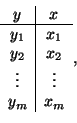
First we will show how to set up the design matrix when there is a
single independent variable involved.
If we are given the data,
and the function we wish to fit using least squares is,
then
The column of 1s in X represents
 . .
If the equation we wanted to fit was quadratic,
then
If the equation was
then
In general, for the table of data,
and any function that is linear with respect to the
coefficients,
then

no_titleno_title
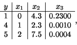
If we are given a dataset that contains multiple independent
variables, for example:
and we want to find a fit for the function
then you would end up with
no_titleno_title
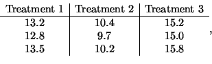
Sometimes the independent variable is a list of treatments and the
dependent variable consists of a list of values measured after each
treatment. For example, if you have the data set,
we can still use a linear model,
and estimate the parameters  , ,  and and  .
However, in this case, .
However, in this case,  consists of a 0 or a 1, depending on which
treatment a given consists of a 0 or a 1, depending on which
treatment a given  value was collected from. Thus,
For a discussion of alternative design matrices (some of which are used, for
historical reasons, more often than this one) for this type of data set, see
Appendix E. value was collected from. Thus,
For a discussion of alternative design matrices (some of which are used, for
historical reasons, more often than this one) for this type of data set, see
Appendix E.
Next: Parameter Estimation: The Least
Up: Linear Models
Previous: General Overview
Index
Click for printer friendely version of this HowTo
Frank Starmer
2004-05-19
| |

![$\displaystyle {\bf Y} =
\left [ \begin{array}{cc}
1\\
4\\
5
\end{array} \righ...
...bf X} =
\left [ \begin{array}{cc}
1 & 0\\
1 & 1\\
1 & 2
\end{array} \right].
$](img759.png)
![$\displaystyle {\bf Y} =
\left [ \begin{array}{cc}
1\\
4\\
5
\end{array} \righ...
... [ \begin{array}{ccc}
1 & 0 & 0\\
1 & 1 & 1\\
1 & 2 & 4
\end{array} \right].
$](img762.png)
![$\displaystyle {\bf Y} =
\left [ \begin{array}{cc}
1\\
4\\
5
\end{array} \righ...
...egin{array}{cc}
\sin(0) & 0\\
\sin(1) & 1\\
\sin(2) & 4
\end{array} \right].
$](img764.png)
![$\displaystyle {\bf X} =
\left [ \begin{array}{cccc}
f_0(x_0) & f_1(x_0) & \cdot...
...ddots & \vdots\\
f_0(x_m) & f_1(x_m) & \cdots & f_n(x_m)
\end{array} \right].
$](img767.png)
![$\displaystyle {\bf Y} =
\left [ \begin{array}{c}
1\\
4\\
5
\end{array} \right...
... & 0.2300\\
1 & 1 & 2.3 & 0.0010\\
1 & 2 & 7.5 & 0.0004
\end{array} \right].
$](img770.png)
![$\displaystyle {\bf Y} =
\left [ \begin{array}{c}
13.2\\
12.8\\
13.5\\
10.4\\...
...1 & 0\\
0 & 1 & 0\\
0 & 0 & 1\\
0 & 0 & 1\\
0 & 0 & 1
\end{array} \right].
$](img775.png)